Plotting antenna radiation patterns
#RadioIn a previous post, I already described my Yagi antenna, that I built for the 2-meter band. Now I would like to extend that antenna for the 70-cm band.
The formula for free space propagation loss (FSPL) - ignoring antenna directivity - is
where d is the distance between the transmitter and receiver and f is the
transmission frequency.
Therefore, the free space propagation loss increases by the square of the
frequency.
Assuming that all other conditions remain the same, a transmission at 435 MHz
in the 70-cm band has a free space propagation loss almost 10 times higher than
a transmission at 144 MHz in the 2-m band.
Thus, more gain and consequently more elements are needed for the 70-cm band.
While the dimensions of the four individual elements for the previous antenna were largely determined by trial and error, this would be impractical for more than 4 elements.
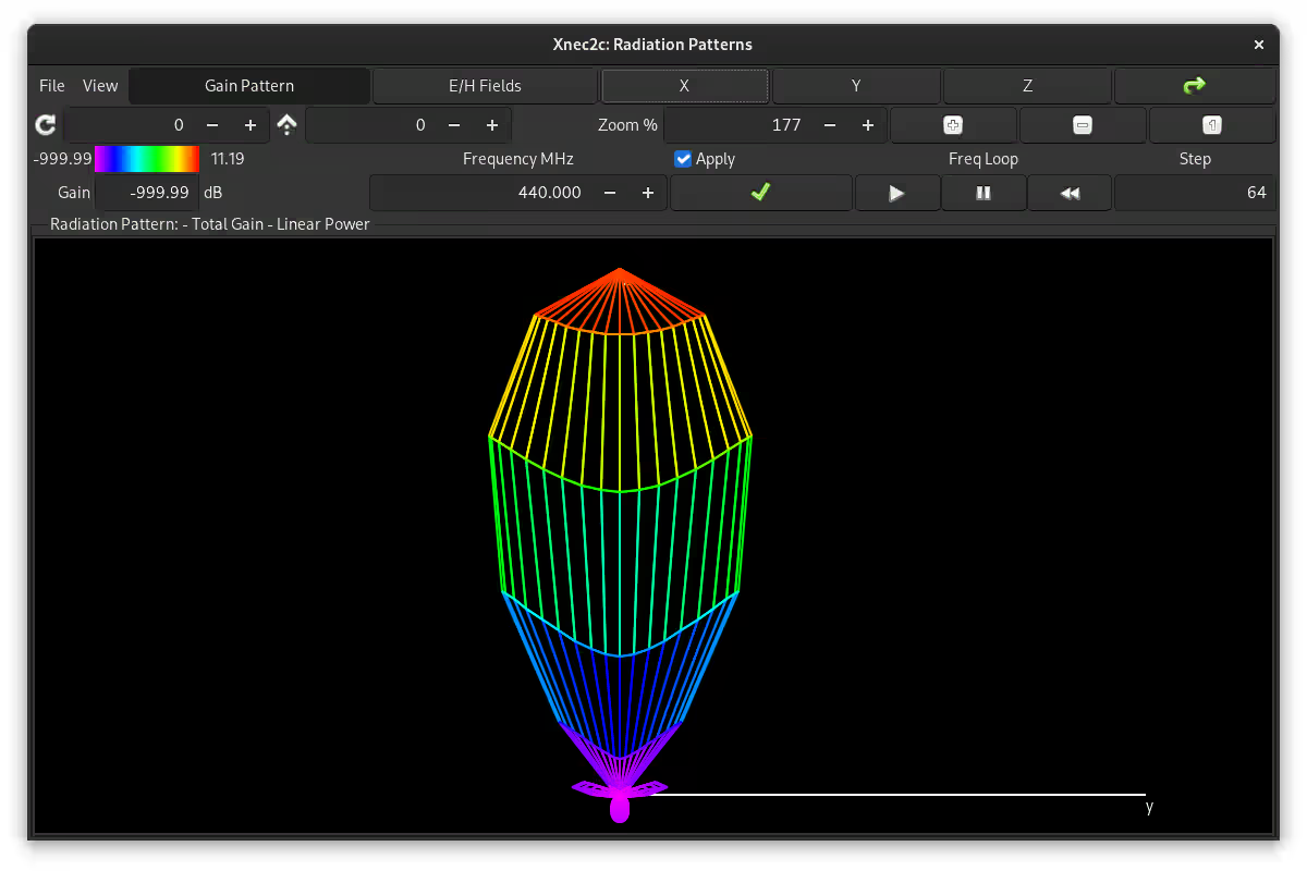
Simulation and optimization in XNEC2C
This is were - once again - xnec2c comes into play. The program is great for simulating antenna characteristics such as gain and SWR. Instead of manually trying out different element positions and lengths, a handy perl script from KJ7LNW - the developer of xnec2c - can be used to optimize the antenna for various parameters like SWR, gain, length or F/B-ratio.
The script xnec2-optimize is really easy to use in combination with xnec2c. Just specify some initial values for element positions and lengths, define the optimization goals - in my case SWR and max gain - and then the script will do a simplex optimization for you.
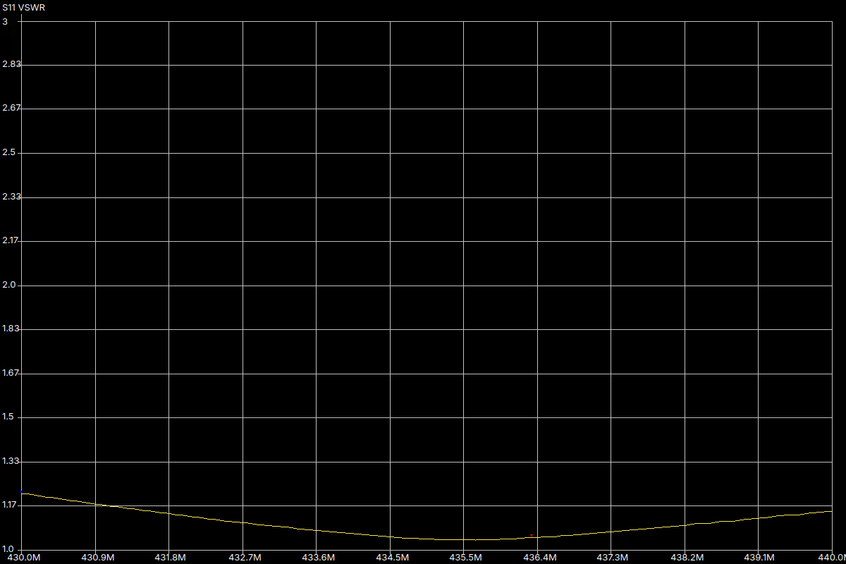
After assembling the antenna, it was already working well and the SWR measurement with a NanoVNA showed promising results. Still, I wanted to check the directivity of the antenna.
A tool to measure antenna directivity
The idea for a tool the measure antenna directivity is simple: A signal source is connected to the antenna, then the antenna is rotated in place while a RTL-SDR is used to measure the received signal strength in an abstract unit.
This abstract unit is called dBFS or decibels relative to the full scale. So what is the full scale? Inside the RTL-SDR is an 8-bit ADC that reads samples from 0 to 255, which are later shifted in software from -128 to 127 (or -127 to 128).
Now let’s take 1000 IQ-samples of two periods of a sine curve from -127 to 127 and observe the result of the fast Fourier transformation. This sine curve saturates the range of the 8-bit ADC without clipping.
import numpy as np
from scipy.signal import hilbert
import matplotlib.pyplot as plt

FFT_SIZE = 1000

t = np.arange(FFT_SIZE)
# Points per periods
ppp = 2 / FFT_SIZE

real = 127 * np.sin(2 * np.pi * ppp * t)
imag = 127j * np.cos(2 * np.pi * ppp * t)

s = real + imag

figure, (time, frequency) = plt.subplots(1, 2, figsize=(12, 6), dpi=100)
time.plot(t, s.real)
time.plot(t, s.imag)
frequency.plot(t, np.abs(np.fft.fftshift(np.fft.fft(s))) / FFT_SIZE)
plt.show()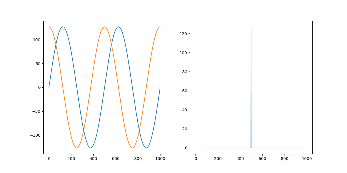
See how the FFT produces a peak at the number_of_periods / FFT_SIZE with an
amplitude of exactly 127.
This is the full scale, so 0 dBFS is 127.
Of course values greater than 0 dBFS are still possible. Let’s have a clipped sine wave with an amplitude greater than 127:
real = 150 * np.sin(2 * np.pi * ppp * t)
imag = 150j * np.cos(2 * np.pi * ppp * t)

s = np.clip(real, -127, 127) + np.clip(imag, -127j, 127j)

figure, (time, frequency) = plt.subplots(1, 2, figsize=(12, 6), dpi=100)
time.plot(t, s.real)
time.plot(t, s.imag)
frequency.plot(t, np.abs(np.fft.fftshift(np.fft.fft(s))) / FFT_SIZE)
plt.show()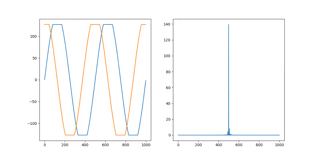
The left plot clearly shows, that the signal is clipped, so the right plot does not show exact frequencies. However, it’s still clear that the peak is above 127.
Finally each value of the FFT result is divided by 127 and then 10 multiplied by the decimal logarithm of the quotient is the value in dBFS.
real = 0.1 * 127 * np.sin(2 * np.pi * ppp * t)
imag = 0.1 * 127j * np.cos(2 * np.pi * ppp * t)

s = real + imag

figure, (time, frequency) = plt.subplots(1, 2, figsize=(12, 6), dpi=100)
time.axis([0, 1000, -127, 127])
time.plot(t, s.real)
time.plot(t, s.imag)
# Clip to -100 dBFS
logmags = np.maximum(
    10 * np.log10(np.abs(np.fft.fftshift(np.fft.fft(s))) / FFT_SIZE / 127),
    -100,
)
frequency.axis([0, 1000, -100, 0])
frequency.plot(t, logmags)
plt.show()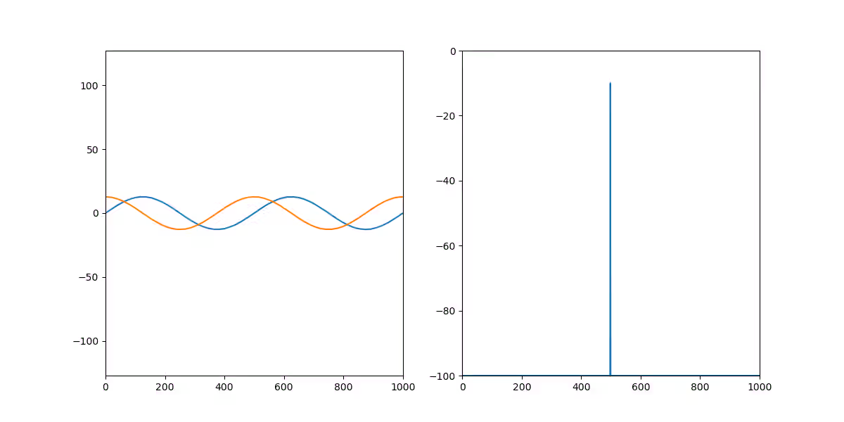
For example, the signal with an amplitude of one tenth of 127 has a signal strength of -10 dBFS.
The tool now consists of two components:
- A backend running on a PC with an RTL-SDR connected a few meters away from the antenna. The backend continuously reads samples from the RTL-SDR and calculates the amplitude at the desired frequency in dBFS.
- A web application running on a mobile device next to the antenna.
Nowadays most mobile devices have built-in orientation sensors like a
compass, so the
DeviceOrientationEventcan be used to get the current antenna rotation. The frontend receives the current amplitude from the backend and uses it in combination with the device rotation to plot a radiation pattern for the antenna.
Implementation and testing took me several weeks.
I settled on Rust for the backend, which I am not that familiar with yet, but
that choice proved to be a great learning opportunity.
Initially I decided against doing the Fourier transformation myself and called
the cli-tool rtl_power from the backend.
However, this had some serious drawbacks, such as only updating the strength of the
received signal once per second, so later I still decided to ditch it and
implemented the sample processing myself.
For the frontend I also decided to dive into some cool new technology and chose Svelte, which afterwards turned out to be a great choice for such a small project.
The tool is called SdrAntennaPatternPlotter and the source code is available for on GitHub. Feel free to check it out.
Using the tool
Apart from a laptop with the RTL-SDR connected and a smartphone mounted on the antenna, there is still the need for a signal source to have an actual signal to measure. Since I have already built many antennas, I have a NanoVNA, which can be misused as a signal source by setting Stimulus -> CW FREQ:
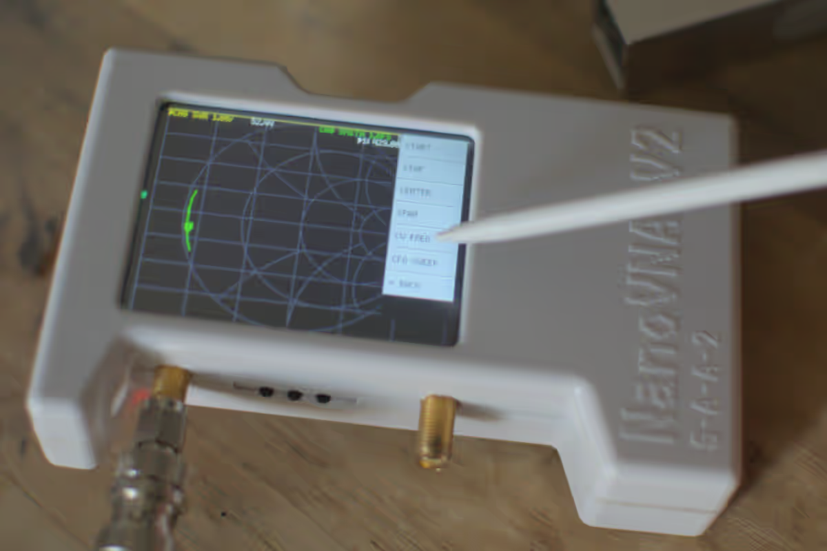
The NanoVNA then outputs a continuous signal with a strength of roughly -10 dBm.
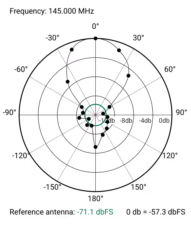
For the actual measurement, the antenna first needs to be assembled, then the laptop with the RTL-SDR gets placed a few meters away. After that first a reference antenna is connected to the signal source. In the following video, the stock antenna of a Yaesu FT-70D handheld transceiver is used. The strength of the signal emitted by the reference antenna will be shown in comparison the the radiation pattern for the antenna to measure. Then the directional antenna is connected to the signal source and the web application instructs how to rotate the antenna for each measurement.
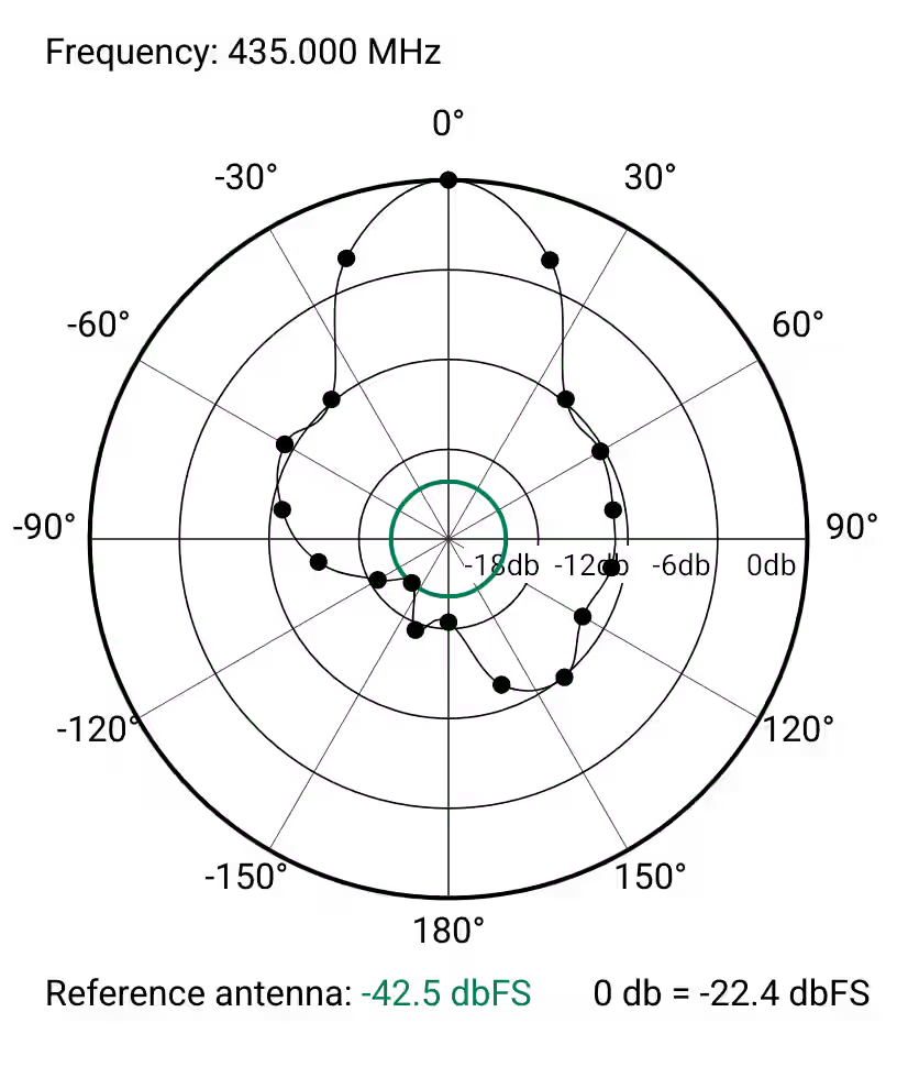
Below are the resulting patterns for both the 2 meter and 70 centimeter band of my new dual band yagi. While the 70 centimeter in particular pattern looks imprecise, there is clearly a significant forward gain visible in both of them.
A word about the results and gain
As mentioned in a previous section, dBFS is still an abstract unit, so any claims about gain, F/B-ratio or similar values based a chart generated by this tool are likely to be foolish.
Still it is useful to verify, that an antenna will indeed radiate in an directional pattern and will beat the stock antenna of my handheld.
Furthermore, I found an interesting post on Google Groups. It talks about the relationship between dBFS as output by Gqrx and the signal strength at the RTL-SDR in dBm. One poster tested the dBFS values in Gqrx against a signal source of known power and discovered, that dBFS is linear to dBm from an input power level between -90 and -40 dBm. As the method of obtaining dBFS in this post is quite similar to that used by Gqrx, the radiation patterns expressed in dBFS should still give a good indication about the gain of the antenna relative to the reference antenna.